Russell Saerang

Graph Realization Made Easy!

This article serves as a detailed breakdown of the code provided in pytils.

Degree Sequence

The degree sequence of a graph is defined as a non-increasing sequence of the graph's vertex degrees, where the degree of a vertex is defined as the number of edges incident to the vertex itself.

Given an undirected graph, constructing the degree sequence is rather easy, if not trivial.

# suppose we represent the graph as an edge list instead of an adjacency list
# vertices are 0-indexed here, get used to it!
N = 5
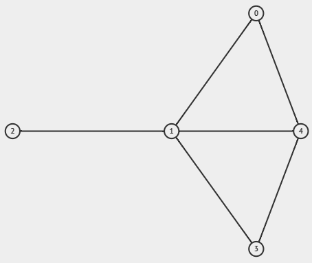
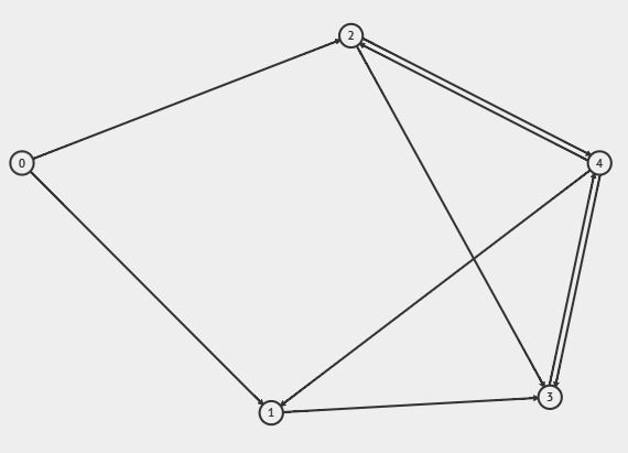
G = [(1, 2), (0, 1), (1, 3), (4, 1), (0, 4), (3, 4)]
D = [0]*N
for a, b in G:
    D[a] += 1; D[b] += 1 # add one to the degree of both endpoint vertices
print(D)                       # [2, 4, 1, 2, 3]
print(sorted(D, reverse=True)) # [4, 3, 2, 2, 1]

Now let's solve the inverse of the problem.

Given a non-increasing array $D$ of size $N$, can we construct an undirected graph with $N$ vertices and degree sequence $D$?

To answer this YES/NO question, we can make use of the Erdős–Gallai theorem that states the following.

The answer is YES if and only if $D_1 + D_2 + \ldots + D_n$ is even and $$\sum_{i=1}^k D_i \le k(k-1) + \sum_{i=k+1}^n \min(D_i, k), \forall 1 \le k \le n$$

The verification in Python is rather straightforward for the left hand side as we make use of the prefix sum. As for the right hand side of the inequality, we can make use of a forward pointer since the degree sequence is non-increasing.

Suppose we have another array $T$ where each of $T_k$ stores the maximum index $i$ of $D$ such that $D_i \ge k$. Then, for a given $k$, we can transform the right hand side as follows.

$$ \begin{align*} \sum_{i=k+1}^n \min(D_i, k) &= \sum_{i=k+1}^{T_k} k + \sum_{i=T_k+1}^{n} D_i \\ &= k(T_k-k) + \sum_{i=T_k+1}^{n} D_i \end{align*} $$

Combining the above equation with the inequality stated by the theorem, we have

$$ \begin{align*} \sum_{i=1}^k D_i &\le k(k-1) + k(T_k-k) + \sum_{i=T_k+1}^{n} D_i \\ &=k(T_k-1) + \sum_{i=T_k+1}^{n} D_i, &\forall 1 \le k \le n \end{align*} $$

# use another non-increasing sequence if necessary
D = [4, 3, 2, 2, 1]
N = len(D)

# create prefix sum for LHS
P = [0]
for d in D:
    P.append(P[-1]+d)

# pointer for RHS
T = [0]*(N+1)
p = 0
for k in range(1, N+1):
    while p < N and D[p] >= k:
        p += 1
    T[k] = p-1

# final result
print(sum(D) % 2 == 0 and all(P[k] <= k*(T[k]-1) + P[N]-P[T[k]] for k in range(1, N+1)))

When the graph is directed, the similar theorem would be the Fulkerson–Chen–Anstee theorem. Suppose you have the degree sequence $D = [(O_1, I_1), (O_2, I_2), \ldots, (O_n, I_n)]$ where $O_1 \ge O_2 \ge \ldots \ge O_n$ are the outdegrees of the vertices in non-increasing order and $I_1, I_2, \ldots, I_n$ are the corresponding vertex indegrees.

The answer is YES if and only if $$\sum_{i=1}^{n} O_i = \sum_{i=1}^{n} I_i$$ and $$\sum_{i=1}^k O_i \le \sum_{i=1}^k \min(I_i, k-1) + \sum_{i=k+1}^n \min(I_i, k), \forall 1 \le k \le n$$

The equivalent Python code is left to you as an exercise, as this is not the main point of the article.

Here's the real challenge: if a construction exists, how do we construct such undirected graph?

Havel-Hakimi Algorithm

Reference Kattis problem: Kjördæmi Königsbergs

If we have to construct the undirected graph, obviously we can't just verify using the Erdős–Gallai theorem. We have to come up with some algorithm to approach this, which is why Havel-Hakimi comes to the rescue.

The algorithm

The ELI5 version of this algorithm is to repetitively pick the vertex with the largest degree, say with a degree of $s$, connect this vertex to the next $s$ vertices with the highest degree, and then update (decrement) the degrees accordingly. In the end, the degree sequence should only consist of zeroes.

Let's take our previous $[4, 3, 2, 2, 1]$ degree sequence as an example. To make things easier, we will assume that the values in $D$ are the degrees of vertices $0, 1, \ldots, n-1$ in that particular order.

• Currently, vertex 0 has the largest degree of 4. We connect 0 to the next 4 vertices with the highest degree: 1, 2, 3, 4.
  • Degree sequence becomes $[0, 2, 1, 1, 0]$.
• Currently, vertex 1 has the largest degree of 2. We connect 0 to the next 2 vertices with the highest degree: 2, 3.
  • Degree sequence becomes $[0, 0, 0, 0, 0]$.
• Our final edge list is $[(0, 1), (0, 2), (0, 3), (0, 4), (1, 2), (1, 3)]$. We are done.

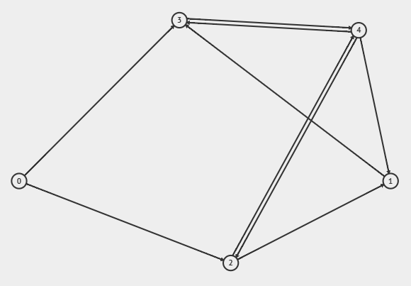
If you noticed, the final result is different than our initial graph $[(1, 2), (0, 1), (1, 3), (4, 1), (0, 4), (3, 4)]$, and this is caused by the pre-sorting of the degree sequence $D$. In fact, even if the initial array is not non-increasing, we can still order the degrees by storing $(D_i, i)$ instead of just $D_i$, and in the end we re-map the indices based on the values of $i$ attached to the $D_i$'s.

Repeating this process, but this time instead of storing $D = [2, 4, 1, 2, 3]$, we have $D = [(2, 0), (4, 1), (1, 2), (2, 3), (3, 4)]$ which is then sorted to be $[(4, 1), (3, 4), (2, 0), (2, 3), (1, 2)]$. Remapping the edge list that we obtained earlier using $[0, 1, 2, 3, 4] \rightarrow [1, 4, 0, 3, 2]$, we get $[(1, 4), (1, 0), (1, 3), (1, 2), (4, 0), (4, 3)]$, which is finally the same as our initial graph.

Another thing that I'd like to point out is that the construction is not unique. The degree sequence $[1, 1, 1, 1, 1, 1]$ can be obtained from any edge-pairing of the 6 vertices in the graph, and there is more than one configuration of the final matching.

Time to implement this in Python using max priority queues. Every time we select the vertex with the largest degree $d$, we store the next $d$ vertices into a temporary queue first (otherwise we might select the same vertex multiple times), and after connecting the edges accordingly we re-enqueue them.

# use another non-increasing sequence if necessary
D = [4, 3, 2, 2, 1]
N = len(D)

# convert to (-D_i, i)
# -D_i instead of D_i due to heapq using min priority queue
D = [(-D[i], i) for i in range(N)]
E = [] # the final edge list

# convert D to priority queue
from heapq import *
heapify(D)

while D:
    d, i = heappop(D)       # d < 0
    tmp = []
    for _ in range(-d):
        assert D            # cannot find such construction
        e, j = heappop(D)   # e < 0
        tmp.append((e+1, j))
        E.append((i, j))
    while tmp:
        heappush(D, tmp.pop()) # re-enqueue everything in tmp

print(E) # [(0, 1), (0, 2), (0, 3), (0, 4), (1, 2), (1, 3)]

The code pushes/pops from the priority queue for a total of $O(m+n)$ times ($O(m)$ from the one inside the for loop and the while tmp loop, $O(n)$ from the main heappop), where $m$ is the number of edges in the graph, and since there are $O(n)$ elements in the priority queue, the runtime of this code is $O((m+n) \log n)$.

Ensuring connectivity

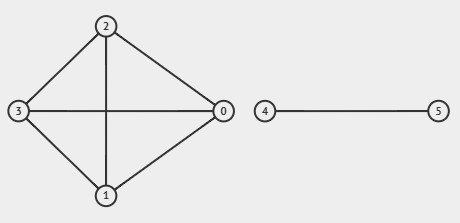
This algorithm, however, has a problem when it comes to ensuring the connectivity of the graph. Consider the degree sequence $[3, 3, 3, 3, 1, 1]$. Using the above algorithm, we get $[(0, 1), (0, 2), (0, 3), (1, 2), (1, 3), (2, 3), (4, 5)]$ as our final edge list of an (apparently) unconnected graph! However, the graph $[(3, 5), (2, 4), (1, 2), (0, 2), (0, 1), (3, 1), (3, 0)]$ is a connected graph that yields the same degree sequence!

The trick here is to change on how we select the pivot vertex. Turns out, if you always pick the vertex with the smallest nonzero degree $d$, but you still connect this with the top $d$ vertices with the largest degree, you actually still get a valid construction. However, in this approach, we are minimizing the number of small components formed by pairing small-degree vertices with small-degree vertices, and therefore increasing our chances of obtaining a connected graph. An edge case to consider is when $\sum_{i=1}^n D_i < 2n-2$, to which the graph will not be connected however we arrange the edges.

Let's use this new approach on the degree sequence $[3, 3, 3, 3, 1, 1]$. Note that there is no need for a tiebreaker: you just need to ensure the vertices selected has indeed the largest/smallest degrees.

• Pick smallest-degree vertex: 5. Pick top-1 largest-degree vertex: $[0]$. Add $(0, 5)$ to edge list.
  • Degree sequence is now $[2, 3, 3, 3, 1, 0]$.
• Pick smallest-degree vertex: 4. Pick top-1 largest-degree vertex: $[1]$. Add $(1, 4)$ to edge list.
  • Degree sequence is now $[2, 2, 3, 3, 0, 0]$.
• Pick smallest-degree vertex: 0. Pick top-2 largest-degree vertex: $[2, 3]$. Add $(0, 2)$ and $(0, 3)$ to edge list.
  • Degree sequence is now $[0, 2, 2, 2, 0, 0]$.
• Pick smallest-degree vertex: 1. Pick top-2 largest-degree vertex: $[2, 3]$. Add $(1, 2)$ and $(1, 3)$ to edge list.
  • Degree sequence is now $[0, 0, 1, 1, 0, 0]$.
• Pick smallest-degree vertex: 2. Pick top-1 largest-degree vertex: $[3]$. Add $(2, 3)$ to edge list.
  • Degree sequence is now $[0, 0, 0, 0, 0, 0]$. We are done.

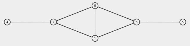
Notice that the resulting graph $[(0, 5), (1, 4), (0, 2), (0, 3), (1, 2), (1, 3), (2, 3)]$ is indeed connected, which leaves us with the challenge to implement this in Python. Since we now need to take the smallest as well as the largest out of the data structure, simply using a priority queue won't suffice to maintain the time complexity. You can either use a custom-made BST or using the SortedList template (the latter is theoretically not $O(\log n)$ per query, but has been made fast enough to approach this time complexity).

... # paste the whole SortedList class here

# use another non-increasing sequence if necessary
D = [4, 3, 2, 2, 1]
N = len(D)

# convert to (D_i, i)
D = SortedList([(D[i], i) for i in range(N)])
E = [] # the final edge list

tmp = []
while D:
    d, i = D.pop(0)
    for _ in range(d):
        assert D
        e, j = D.pop()
        tmp.append((e-1, j))
        E.append((i, j))
    while tmp:
        D.append(tmp.pop()) # re-enqueue everything in tmp

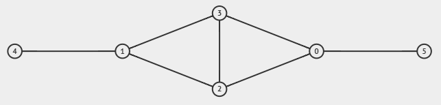
print(E) # [(4, 0), (2, 1), (2, 0), (0, 3), (0, 1), (1, 3)]

With the same reasoning as our previous Python code, the runtime of this code is $O((m+n) \log n)$, where $m, n$ are respectively the number of edges and vertices in the graph.

Improving the runtime

We can actually improve the runtime from $O((m+n) \log n)$ to just $O(m+n)$!

In order to do so, we make use of the degree buckets: use an array of arrays $Q$ where $Q_i$ stores the vertices with degree $i$ at the moment. Then, we keep track of a pointer $L$ for the position of the smallest-degree vertex and another pointer $R$ for the largest-degree vertex. I wanted to give a pseudocode but I think the comments within the code below are sufficient.

# use another non-increasing sequence if necessary
D = [4, 3, 2, 2, 1]
N = len(D)
E = [] # the final edge list

# buckets
Q = [[] for _ in range(max(D)+1)]
for i in range(N):
    Q[D[i]].append(i)

# two pointers
L = 1
R = len(Q)-1
tmp = []
while L <= R:
    # increment L until we find a vertex with degree L
    if not Q[L]:
        L += 1
        continue

    # there is at least one vertex of degree L
    v = Q[L].pop()

    # decrement R until we find a vertex with degree R
    while R and not Q[R]:
        R -= 1

    # We can't decrement R inside the for loop
    # Let's say we will take vertices of degrees (x-3, x-2, x) -> (x-4, x-3, x-1)
    # If we keep decrementing R, in the end of this iteration we will get R <= x-3
    # But there is still a vertex with degree x-1, so R will be incorrect
    # Let's have a copy of R called S that we'll keep decrementing instead of R
    # Then after the iteration we will go back from S to R
    # TLDR: R must always keep track of the largest-degree vertex
    S = R

    # find the L largest-degree vertices
    for _ in range(L):
        # decrement S until we find a vertex with degree S
        while S and not Q[S]:
            S -= 1

        assert S > 0 # we must find a nonzero-degree vertex

        u = Q[S].pop()
        E.append((u, v))
        if S > 1:
            tmp.append((u, S-1))

    # re-enqueue everything from tmp
    while tmp:
        u, x = tmp.pop()
        Q[x].append(u)

    # What happens when L == S here?
    # We will re-enqueue something to Q[S-1], so we have to pull back L by 1 step
    # Otherwise, some re-enqueued vertices will be ignored
    # TLDR: L must always keep track of the smallest-degree vertex
    if L == S:
        L -= 1

print(E) # [(0, 4), (0, 3), (1, 3), (1, 0), (2, 0), (2, 1)]

Analyzing the time complexity, we can see that using the buckets, we have cut down the $O(\log n)$ factor. The $O(m+n)$ is due to the fact that there are $O(m+n)$ appends and pops from this data structure, the $L$ pointer only moves at most $O(m+n)$ steps to the right (even with the L == S case), and the $R$ pointer moves at most $O(n)$ steps to the left.

There is still one last problem. There can be a case where $L$ is sufficiently high that the value of $S$ before and after you find the $L$ vertices are very far away, and therefore when processing the next smallest-degree vertex, you have to redo this journey again from $S_{\text{before}}$ to $S_{\text{after}}$, while every bucket in between might've been empty. To optimize this, we can have a "jump array" called $J$ that stores where to jump from a particular index $k$ in $Q$ instead of always being $k-1$.

Let's say we during the journey from $S = S_{\text{before}}$ to $S = S_{\text{after}}$, we have a bunch of indices with vertices that we selected to connect with $S_1 \ge S_2 \ge \ldots \ge S_L$. We can update the value of $J_{S_i}$ for $i = 1, 2, \ldots, L$ into $J_{J_{S_i}}$. For large gaps, the total number of steps will be expected to half every time it gets explored.

Another edge case is when we have put $J_{s}$ for some $s$ into something that is less than $s-1$, but after taking a degree of a vertex in $Q[s]$, we need to relocate this vertex to $s-1$. This means we have to be able to undo our update of $J_{s}$ back to $s-1$ and $J_{s-1}$ to the old $J_{s}$.

The time complexity remains the same, but the constant factor will get better. With this, behold the final version of the Havel-Hakimi algorithm.

D = [4, 3, 2, 2, 1]

N = len(D)
E = [] # the final edge list

# buckets
Q = [[] for _ in range(max(D)+1)]
for i in range(N):
    Q[D[i]].append(i)

# two pointers
L = 1
R = len(Q)-1
tmp = []

# initial jump array: from x to x-1
J = [i-1 for i in range(R+1)]

while L <= R:
    # increment L until we find a vertex with degree L
    if not Q[L]:
        L += 1
        continue

    v = Q[L].pop() # there is at least one vertex of degree L
    B = [] # which indices of J to update
    S = R

    # find the L largest-degree vertices
    for _ in range(L):
        # go to next value of S until we find a vertex with degree S
        while S and not Q[S]:
            B.append(S) # update the value of J[S] later
            S = J[S]

        assert S > 0 # we must find a nonzero-degree vertex

        u = Q[S].pop()
        E.append((u, v))
        if S > 1:
            tmp.append((u, S-1))

    while tmp:
        u, x = tmp.pop()
        if J[x+1] != x: # undo update of J
            J[x], J[x+1] = J[x+1], x
        Q[x].append(u)

    # close the gaps
    for b in B:
        if not Q[J[b]]:
            J[b] = J[J[b]]

    if L == S:
        L -= 1

print(E) # [(0, 4), (0, 3), (1, 3), (1, 0), (2, 0), (2, 1)]

Kleitman-Wang Algorithm

Reference Kattis problem: Follower Forensics

We can use the idea from the optimized Havel-Hakimi algorithm to solve the case when the graph is directed and we're given two arrays instead: the outdegree array and the indegree array.

Instead of just ensuring connectivity, we get to be more specific: weak-connectivity. The algorithm is expected to generate a weak-connected graph whenever possible, i.e. when you convert all the directed edges into undirected, the graph becomes connected.

Instead of just selecting the smallest-degree vertex, we select the smallest-outdegree/indegree vertex (obviously ignoring those with degree of 0), whichever has a smaller such degree of $d$ (if they are the same, take the outdegree first). This means we take $d$ vertices with the highest indegree/outdegree, and update their degrees accordingly after connecting them with the proper directed edges.

For example, we start with a graph of 5 vertices with the outdegree $O = [2, 1, 2, 1, 3]$ and the indegree $I = [0, 2, 2, 3, 2]$.

• Smallest outdegree = 1 at vertex 1, smallest indegree = 2 at vertex 1, this means we process vertex 1.
  • Pick top-1 largest indegree vertex: 3. Add $1 \rightarrow 3$ to edge list.
  • $O$ is now $[2, 0, 2, 1, 3]$, $I$ is now $[0, 2, 2, 2, 2]$.
• Smallest outdegree = 1 at vertex 3, smallest indegree = 2 at vertex 1, this means we process vertex 3.
  • Pick top-1 largest indegree vertex: 1. Add $3 \rightarrow 1$ to edge list.
  • $O$ is now $[2, 0, 2, 0, 3]$, $I$ is now $[0, 1, 2, 2, 2]$.
• Smallest outdegree = 2 at vertex 0, smallest indegree = 1 at vertex 1, this means we process vertex 1.
  • Pick top-1 largest outdegree vertex: 4. Add $4 \rightarrow 1$ to edge list.
  • $O$ is now $[2, 0, 2, 0, 2]$, $I$ is now $[0, 0, 2, 2, 2]$.
• Smallest outdegree = 2 at vertex 0, smallest indegree = 2 at vertex 2, this means we process vertex 0.
  • Pick top-2 largest indegree vertex: 2 and 3. Add $0 \rightarrow 2$ and $0 \rightarrow 3$ to edge list.
  • We could've picked 0 instead of 2 or 3, but since the vertex we're processing is 0, we need to refrain from making a self-loop.
  • $O$ is now $[0, 0, 2, 0, 2]$, $I$ is now $[0, 0, 2, 1, 1]$.
• Smallest outdegree = 2 at vertex 2, smallest indegree = 1 at vertex 3, this means we process vertex 3.
  • Pick top-1 largest outdegree vertex: 2. Add $2 \rightarrow 3$ to edge list.
  • $O$ is now $[0, 0, 1, 0, 2]$, $I$ is now $[0, 0, 2, 0, 1]$.
• Smallest outdegree = 1 at vertex 2, smallest indegree = 1 at vertex 4, this means we process vertex 2.
  • Pick top-1 largest indegree vertex: 2. Since the processed vertex is also 2, we skip this and take the next largest: 4. Add $2 \rightarrow 4$ to edge list.
  • $O$ is now $[0, 0, 0, 0, 2]$, $I$ is now $[0, 0, 2, 0, 0]$.
• Now we have 2 outgoing edges from vertex 4 to vertex 2, which means something is wrong (the input is supposed to be a valid graph degree array).

Fixing the tiebreaker

So what went wrong? The tiebreaker for selecting the largest/smallest degree vertices was fixated on whichever has the smaller vertex label, so maybe this wasn't the best strategy. Using the same logic, if we fix both selection tiebreakers on whichever has the larger vertex label, the same outcome might happen.

The next intuitive tiebreaker would be to break the ties on largest degrees by larger vertex number, and smallest degrees by smaller vertex number. This means we can represent the degrees as $(D_i, i)$ instead of just $D_i$ for easier readability.

Start with the same graph of 5 vertices with the outdegree $O = [(2, 0), (1, 1), (2, 2), (1, 3), (3, 4)]$ and the indegree $I = [(2, 1), (2, 2), (3, 3), (2, 4)]$. (vertices with 0 degree ignored)

• Smallest outdegree = $(1, 1)$, smallest indegree = $(2, 1)$, this means we process vertex 1.
  • Pick top-1 largest indegree vertex: $(3, 3)$. Add $1 \rightarrow 3$ to edge list.
  • $O$ is now $[(2, 0), (2, 2), (1, 3), (3, 4)]$, $I$ is now $[(2, 1), (2, 2), (2, 3), (2, 4)]$.
• Smallest outdegree = $(1, 3)$, smallest indegree = $(2, 1)$, this means we process vertex 3.
  • Pick top-1 largest indegree vertex: $(2, 4)$. Add $3 \rightarrow 4$ to edge list.
  • $O$ is now $[(2, 0), (2, 2), (3, 4)]$, $I$ is now $[(2, 1), (2, 2), (2, 3), (1, 4)]$.
• Smallest outdegree = $(2, 0)$, smallest indegree = $(1, 4)$, this means we process vertex 4.
  • Pick top-1 largest outdegree vertex: $(3, 4)$. Since the processed vertex is 4, we avoid self-loop and take the next largest: $(2, 2)$. Add $2 \rightarrow 4$ to edge list.
  • $O$ is now $[(2, 0), (1, 2), (3, 4)]$, $I$ is now $[(2, 1), (2, 2), (2, 3)]$.
• Smallest outdegree = $(1, 2)$, smallest indegree = $(2, 1)$, this means we process vertex 2.
  • Pick top-1 largest indegree vertex: $(2, 3)$. Add $2 \rightarrow 3$ to edge list.
  • $O$ is now $[(2, 0), (3, 4)]$, $I$ is now $[(2, 1), (2, 2), (1, 3)]$.
• Smallest outdegree = $(2, 0)$, smallest indegree = $(1, 3)$, this means we process vertex 3.
  • Pick top-1 largest outdegree vertex: $(3, 4)$. Add $4 \rightarrow 3$ to edge list.
  • $O$ is now $[(2, 0), (2, 4)]$, $I$ is now $[(2, 1), (2, 2)]$.
• Smallest outdegree = $(2, 0)$, smallest indegree = $(2, 4)$, this means we process vertex 0.
  • Pick top-2 largest indegree vertex: $(2, 1)$ and $(2, 2)$. Add $0 \rightarrow 1$ and $0 \rightarrow 2$ to edge list.
  • $O$ is now $[(2, 4)]$, $I$ is now $[(1, 1), (1, 2)]$.
• Smallest outdegree = $(2, 4)$, smallest indegree = $(1, 1)$, this means we process vertex 1.
  • Pick top-1 largest outdegree vertex: $(2, 4)$. Add $4 \rightarrow 1$ to edge list.
  • $O$ is now $[(1, 4)]$, $I$ is now $[(1, 2)]$.
• Add $4 \rightarrow 2$ to edge list.
• We end up with this adjacency list: $0 \rightarrow [1, 2], 1 \rightarrow [3], 2 \rightarrow [3, 4], 3 \rightarrow [4], 4 \rightarrow [1, 2, 3]$, which is indeed a valid weak-connected directed graph.

Let's try another example with $O = [(3, 0), (3, 1), (2, 2), (1, 3), (1, 4)]$ and $I = [(1, 0), (2, 1), (3, 2), (2, 3), (2, 4)]$.

• Smallest outdegree = $(1, 3)$, smallest indegree = $(1, 0)$, this means we process vertex 3.
  • Pick top-1 largest indegree vertex: $(3, 2)$. Add $3 \rightarrow 2$ to edge list.
  • $O$ is now $[(3, 0), (3, 1), (2, 2), (1, 4)]$, $I$ is now $[(1, 0), (2, 1), (2, 2), (2, 3), (2, 4)]$.
• Smallest outdegree = $(1, 4)$, smallest indegree = $(1, 0)$, this means we process vertex 4.
  • Pick top-1 largest indegree vertex (skip 4): $(2, 3)$. Add $4 \rightarrow 3$ to edge list.
  • $O$ is now $[(3, 0), (3, 1), (2, 2)]$, $I$ is now $[(1, 0), (2, 1), (2, 2), (1, 3), (2, 4)]$.
• Smallest outdegree = $(2, 2)$, smallest indegree = $(1, 0)$, this means we process vertex 0.
  • Pick top-1 largest outdegree vertex: $(3, 1)$. Add $1 \rightarrow 0$ to edge list.
  • $O$ is now $[(3, 0), (2, 1), (2, 2)]$, $I$ is now $[(2, 1), (2, 2), (1, 3), (2, 4)]$.
• Smallest outdegree = $(2, 1)$, smallest indegree = $(1, 3)$, this means we process vertex 3.
  • Pick top-1 largest outdegree vertex: $(3, 0)$. Add $0 \rightarrow 3$ to edge list.
  • $O$ is now $[(2, 0), (2, 1), (2, 2)]$, $I$ is now $[(2, 1), (2, 2), (2, 4)]$.
• Smallest outdegree = $(2, 0)$, smallest indegree = $(2, 1)$, this means we process vertex 0.
  • Pick top-2 largest indegree vertex: $(2, 2)$ and $(2, 4)$. Add $0 \rightarrow 2$ and $0 \rightarrow 4$ to edge list.
  • $O$ is now $[(2, 1), (2, 2)]$, $I$ is now $[(2, 1), (1, 2), (1, 4)]$.
• Smallest outdegree = $(2, 1)$, smallest indegree = $(1, 2)$, this means we process vertex 2.
  • Pick top-1 largest outdegree vertex: $(2, 1)$ (skip 2). Add $2 \rightarrow 1$ to edge list.
  • $O$ is now $[(1, 1), (2, 2)]$, $I$ is now $[(2, 1), (1, 4)]$.
• To avoid self-loop, the $(1, 1)$ in $O$ would mean we must have $1 \rightarrow 4$, which will make us end with $O = [(2, 2)]$ and $I = [(2, 1)]$... a double-edge! This means our tiebreaker isn't perfect yet!

Instead of doing the previous two tiebreakers, we should be doing this: while selecting the smallest/largest indegree/outdegree vertex, break ties by selecting the one with larger outdegree/indegree.

Starting with the first one: $O = [(2, 0), (1, 1), (2, 2), (1, 3), (3, 4)]$ and $I = [(2, 1), (2, 2), (3, 3), (2, 4)]$.

• Smallest outdegree = $(1, 3)$ (instead of vertex 1 since vertex 3 has a larger indegree), smallest indegree = $(2, 4)$ (same reasoning), this means we process vertex 3.
  • Pick top-1 largest indegree vertex: $(2, 4)$ (avoid 3). Add $3 \rightarrow 4$ to edge list.
  • $O$ is now $[(2, 0), (1, 1), (2, 2), (3, 4)]$, $I$ is now $[(2, 1), (2, 2), (3, 3), (1, 4)]$.
• Smallest outdegree = $(1, 1)$, smallest indegree = $(1, 4)$, this means we process vertex 1.
  • Pick top-1 largest indegree vertex: $(3, 3)$. Add $1 \rightarrow 3$ to edge list.
  • $O$ is now $[(2, 0), (2, 2), (3, 4)]$, $I$ is now $[(2, 1), (2, 2), (2, 3), (1, 4)]$.
• Smallest outdegree = $(2, 2)$ (vertex 2 has larger indegree than vertex 0), smallest indegree = $(1, 4)$, this means we process vertex 4.
  • Pick top-1 largest outdegree vertex: $(2, 2)$ (vertex 2 still has larger indegree than vertex 0). Add $2 \rightarrow 4$ to edge list.
  • $O$ is now $[(2, 0), (1, 2), (3, 4)]$, $I$ is now $[(2, 1), (2, 2), (2, 3)]$.
• Smallest outdegree = $(1, 2)$, smallest indegree = $(2, 2)$ (vertex 2 has the largest outdegree among vertices 1, 2, 3), this means we process vertex 2.
  • Pick top-1 largest indegree vertex: $(2, 1)$ (same reasoning as above, but you avoid picking 2 again). Add $2 \rightarrow 1$ to edge list.
  • $O$ is now $[(2, 0), (3, 4)]$, $I$ is now $[(1, 1), (2, 2), (2, 3)]$.
• Smallest outdegree = $(2, 0)$, smallest indegree = $(1, 1)$, this means we process vertex 1.
  • Pick top-1 largest outdegree vertex: $(3, 4)$. Add $4 \rightarrow 1$ to edge list.
  • $O$ is now $[(2, 0), (2, 4)]$, $I$ is now $[(2, 2), (2, 3)]$.
• Smallest outdegree = $(2, 0)$ (or vertex 4 is also fine since their indegrees are both 0), smallest indegree = $(2, 2)$ (or vertex 3 is also fine since their outdegrees are both 0), this means we process vertex 0.
  • Pick top-2 largest indegree vertex: $(2, 2)$ and $(2, 3)$. Add $0 \rightarrow 2$ and $0 \rightarrow 3$ to edge list.
  • $O$ is now $[(2, 4)]$, $I$ is now $[(1, 2), (1, 3)]$.
• Smallest outdegree = $(2, 4)$, smallest indegree = $(1, 2)$ (or vertex 3 is also fine), this means we process vertex 2.
  • Pick top-1 largest outdegree vertex: $(2, 4)$. Add $4 \rightarrow 2$ to edge list.
  • $O$ is now $[(1, 4)]$, $I$ is now $[(1, 3)]$.
• Final step connects $4 \rightarrow 3$, both $O$ and $I$ are now empty.
• We end up with this adjacency list: $0 \rightarrow [2, 3], 1 \rightarrow [3], 2 \rightarrow [1, 4], 3 \rightarrow [4], 4 \rightarrow [1, 2, 3]$, which is indeed a valid weak-connected directed graph.

Next one is $O = [(3, 0), (3, 1), (2, 2), (1, 3), (1, 4)]$ and $I = [(1, 0), (2, 1), (3, 2), (2, 3), (2, 4)]$.

• Smallest outdegree = $(1, 3)$ (vertex 4 has the same indegree AND outdegree as vertex 3, so the choice between 3 or 4 doesn't matter here), smallest indegree = $(1, 0)$, this means we process vertex 3.
  • Pick top-1 largest indegree vertices: $(3, 2)$. Add $3 \rightarrow 2$ to edge list.
  • $O$ is now $[(3, 0), (3, 1), (2, 2), (1, 4)]$, $I$ is now $[(1, 0), (2, 1), (2, 2), (2, 3), (2, 4)]$.
• Smallest outdegree = $(1, 4)$, smallest indegree = $(1, 0)$, this means we process vertex 4.
  • Pick top-1 largest indegree vertices: $(2, 1)$ (break ties by largest outdegree as usual). Add $4 \rightarrow 1$ to edge list.
  • $O$ is now $[(3, 0), (3, 1), (2, 2)]$, $I$ is now $[(1, 0), (1, 1), (2, 2), (2, 3), (2, 4)]$.
• Smallest outdegree = $(2, 2)$, smallest indegree = $(1, 0)$ (tie between vertex 0 and 1, but any choice doesn't matter), this means we process vertex 0.
  • Pick top-1 largest outdegree vertices: $(3, 1)$ (another tie between vertex 0 and 1, just avoid self-loop). Add $1 \rightarrow 0$ to edge list.
  • $O$ is now $[(3, 0), (2, 1), (2, 2)]$, $I$ is now $[(1, 1), (2, 2), (2, 3), (2, 4)]$.
• Smallest outdegree = $(2, 2)$ (apply tiebreaker rules), smallest indegree = $(1, 1)$, this means we process vertex 1.
  • Pick top-1 largest outdegree vertices: $(3, 0)$. Add $0 \rightarrow 1$ to edge list.
  • $O$ is now $[(2, 0), (2, 1), (2, 2)]$, $I$ is now $[(2, 2), (2, 3), (2, 4)]$.
• Smallest outdegree = $(2, 2)$ (apply tiebreaker rules), smallest indegree = $(2, 2)$ (apply tiebreaker rules), this means we process vertex 2.
  • Pick top-2 largest indegree vertices: $(2, 3)$ and $(2, 4)$ (avoid vertex 2). Add $2 \rightarrow 3$ and $2 \rightarrow 4$ to edge list.
  • $O$ is now $[(2, 0), (2, 1)]$, $I$ is now $[(2, 2), (1, 3), (1, 4)]$.
• Smallest outdegree = $(2, 1)$ (either vertex 0 or vertex 1 doesn't matter since their indegrees are both 0), smallest indegree = $(1, 3)$ (either vertex 3 or 4 is fine since their outdegrees are both 0), this means we process vertex 3.
  • Pick top-1 largest outdegree vertices: $(2, 1)$ (or again, vertex 0 is also fine). Add $1 \rightarrow 3$ to edge list.
  • $O$ is now $[(2, 0), (1, 1)]$, $I$ is now $[(2, 2), (1, 4)]$.
• Smallest outdegree = $(1, 1)$, smallest indegree = $(1, 4)$, this means we process vertex 1.
  • Pick top-1 largest indegree vertices: $(2, 2)$. Add $1 \rightarrow 2$ to edge list.
  • $O$ is now $[(2, 0)]$, $I$ is now $[(1, 2), (1, 4)]$.
• Smallest outdegree = $(2, 0)$, smallest indegree = $(1, 2)$ (either vertex 2 or 4 is fine since their outdegrees are both 0), this means we process vertex 2.
  • Pick top-1 largest outdegree vertices: $(2, 0)$. Add $0 \rightarrow 2$ to edge list.
  • $O$ is now $[(1, 0)]$, $I$ is now $[(1, 4)]$.
• Final step connects $0 \rightarrow 4$, both $O$ and $I$ are now empty.
• We end up with this adjacency list: $0 \rightarrow [1, 2, 4], 1 \rightarrow [0, 2, 3], 2 \rightarrow [3, 4], 3 \rightarrow [2], 4 \rightarrow [1]$, which is indeed a valid weak-connected directed graph.

Python code

The code has a lot of similarities with the Havel-Hakimi version, but now we have two degree buckets: one for outdegree, and one for indegree. Since we want to handle the tiebreaker, store the indegree in decreasing order on the outdegree bucket and vice versa for the other degree bucket using priority queues as shown below.

# make sure that len(O) == len(I)
O = [3, 3, 2, 1, 1]
I = [1, 2, 3, 2, 2]

N = len(O)
E = [] # the final edge list

# pointers and buckets
L = 1
R = max(O+I)
P = [[] for _ in range(R+1)] # for outdegree
Q = [[] for _ in range(R+1)] # for indegree
from heapq import *
for i in range(N):
    P[O[i]].append((-I[i], i)) # decreasing indegree within the same outdegree
    Q[I[i]].append((-O[i], i)) # decreasing outdegree within the same indegree
for i in range(R+1):
    heapify(P[i]) # convert both to PQ
    heapify(Q[i])

# jump array and tmp for re-enqueue
J = [i-1 for i in range(R+1)]
tmp = []

while L <= R:
    # cannot find any vertex with in/outdegree L, check *both* P[L] and Q[L]
    if not P[L] and not Q[L]:
        L += 1; continue

    # Should we process indegree or outdegree?
    # If indegree, we simply swap the buckets along with the indegree/outdegree arrays
    # This is so that without loss of generality, we'll always take the smallest from P and the largest from Q
    swap = not P[L]
    if swap:
        P, Q, O, I = Q, P, I, O

    _, v = heappop(P[L])
    B = []
    S = R
    pos_v = 0

    for _ in range(L):
        # We try to skip if Q[S] only contains vertex v or is empty
        # If v is found anywhere in Q[S], we will pop it first, and then get the next vertex
        # There is definitely another vertex within Q[S] that is not v
        # If we popped v from Q[S] at some time, add it back (use the pos_v variable) after finding the L vertices
        while S and (not Q[S] or (len(Q[S]) == 1 and Q[S][0][1] == v)):
            B.append(S)
            S = J[S]

        assert S > 0

        _, u = heappop(Q[S])
        if u == v:
            _, u = heappop(Q[S])
            pos_v = S
        E.append((u, v) if swap else (v, u))
        O[v] -= 1 # update outdegree
        I[u] -= 1 # update indegree
        if S > 1:
            tmp.append((u, S-1))

    # re-add v if popped
    if pos_v:
        heappush(Q[pos_v], (-O[v], v))

    while tmp:
        u, x = tmp.pop()
        if J[x+1] != x:
            J[x], J[x+1] = J[x+1], x
        heappush(Q[x], (-O[u], u))

    for b in B:
        if not P[J[b]] and not Q[J[b]]: # check *both* P[J[b]] and Q[J[b]]
            J[b] = J[J[b]]

    if L == S:
        L -= 1

    # revert the swap back to normal
    if swap:
        P, Q, O, I = Q, P, I, O

print(E) # [(3, 2), (4, 1), (1, 0), (0, 1), (2, 3), (2, 4), (1, 3), (1, 2), (0, 2), (0, 4)]

The time complexity is now to $O(m \log n)$ due to the use of priority queues, where $m$ is the number of edges and $n$ is the number of vertices. From what I heard, however, there is a technique to convert this algorithm into linear time like $O(m+n)$, but I'll leave that for the upcoming write-ups.