Russell Saerang

Fast Fourier Transform Made Easy!

Motivation

It all started back in 2021 when I saw this problem on Kattis that asks you to multiply two polynomials. Given the constraints, directly multiplying them (like how people would in mathematics class) should be within the time limit. We can represent the polynomial $P(x) = a_0 + a_1x + a_2x^2 + \ldots + a_{n-1}x^{n-1}$ as a list of $n$ coefficients $[a_0, a_1, a_2, \ldots, a_{n-1}]$, and then a simple Python code like this should do the rest of the trick.

A = [1, 0, 5] # 5x^2 + 1
B = [1, 1]    # x + 1
C = [0]*(len(A)+len(B)-1)

for i in range(len(A)):
    for j in range(len(B)):
        C[i+j] += A[i]*B[j]

print(C) # [1, 1, 5, 5] or 5x^3 + 5x^2 + x + 1

However, when I tried the sequel of the same problem, the code was very much sub-optimal. If the degree of both polynomials are $O(n)$ then the naive algorithm would take $O(n^2)$ time, which will exceed the time limit for $n \approx 10^5$. Even when using Karatsuba's polynomial multiplication, the algorithm will take $O(n^{\log_2 3}) \approx O(n^{1.585})$ time, which at times can also exceed the time limit.

I knew there had to be a "magical" way to solve this problem, and so I found Reducible's video to enlighten me with what people call the Fast Fourier Transform (FFT), and it turned out to be one of my favourite algorithms up to now. Having been about 4.5 years since I watched the video for the first time, I thought I'd give my take on breaking down the algorithm to make it easier to understand.

Fast Fourier Transform (FFT)

Representing polynomials

In the example above, I represented the polynomials using the coefficients, which is the most intuitive way to do so. But, there is another way to represent a polynomial: using the values.

With the fact that we can uniquely represent a polynomial of degree $d$ with $d+1$ distinct points, we can represent $$P(x) = a_0 + a_1x + a_2x^2 + \ldots + a_{n-1}x^{n-1}$$ using $n$ points $$(x_0, P(x_0)), (x_1, P(x_1)), (x_2, P(x_2)), \ldots, (x_{n-1}, P(x_{n-1})).$$ The proof of why the representation exists and is unique revolves around the invertibility of the Vandermonde matrix $V(x_0, x_1, x_2, \ldots, x_{n-1})$.

Now that we use the value representation, multiplying two polynomials will be much easier. Suppose I have two polynomials $A(x)$ and $B(x)$, both with degree $n-1, n \ge 1$ (if they are unequal, pad the one with less degree with 0 coefficients until the degree is also $n-1$). The product will be a polynomial $P(x)$ of degree $2n-2$, which means I need at least $2n-1$ points to uniquely represent $P$. Since $2n-1 \ge n$, we can definitely represent $A$ and $B$ uniquely as well.

Representing both $A$ and $B$ as $$(x_0, A(x_0)), (x_1, A(x_1)), (x_2, A(x_2)), \ldots, (x_{2n-2}, A(x_{2n-2}))$$ and $$(x_0, B(x_0)), (x_1, B(x_1)), (x_2, B(x_2)), \ldots, (x_{2n-2}, B(x_{2n-2}))$$ for some selected values $x_0, x_1, \ldots, x_{2n-2}$, $P$ can be represented as $$(x_0, A(x_0)B(x_0)), (x_1, A(x_1)B(x_1)), (x_2, A(x_2)B(x_2)), \ldots, (x_{2n-2}, A(x_{2n-2})B(x_{2n-2}))$$

For convenience, instead of just fixing one to select $2n-1$ points, we select $N = 2^k$ points for some nonnegative integer $k$ such that $N \ge 2n-1$. This means if our initial polynomials to multiply $A$ and $B$ are of degree $n-1$, we will have to pick $N = 2^{\lceil\log_2(2n)\rceil} = 2^{\lceil\log_2(n)\rceil+1}$ points. (note that $N$ is still $O(n)$)

The next question would be how to bring this value representation back to the polynomial form, and how to select the $N$ values of the $x_i$'s. This is where the FFT algorithm comes in.

While we can solve for the matrix equation shown in the proof using Lagrange polynomials, they are clearly not easy to implement and is still expensive in computation because we have to re-evaluate the polynomial for each $x_i$, which means the total time taken would be still be at least $O(n^2)$.

Odd and even functions

Every polynomial $P(x)$ can be decomposed as a sum of an odd polynomial $O(x)$ and an even polynomial $E(x)$ by looking at the degree of each term in $P(x)$. By definition, we have

$$O(x) = -O(-x), E(x) = E(-x)$$

Once we evaluate $P(x_i) = E(x_i)+O(x_i)$, we can directly infer the value of $P(-x_i) = E(-x_i)-O(-x_i)$ without having to substitute $-x_i$ into $P$. Therefore, we only need to find half as many value as we needed previously: from $N$ to just $\frac{N}{2}$, and then we negate the values to obtain the other half.

Next, notice that $E(x)$ can be represented as a polynomial in terms of $x^2$, meaning there is a polynomial $Q$ (not necessarily odd or even) such that $E(x) = Q(x^2)$. Similarly, $O(x)$ has a factor of $x$ that once factored out can also be represented as a polynomial in terms of $x^2$, meaning there is a polynomial $R$ (also not necessarily odd or even) such that $O(x) = xR(x^2)$. As a result, we obtain the following equations.

$$ P(x_i) = Q(x_i^2) + x_iR(x_i^2) \\ P(-x_i) = Q((-x_i)^2) + -x_iR((-x_i)^2) = Q(x_i^2) - x_iR(x_i^2) $$

For example, if $P(x) = x^3 + 2x^2 - 7x + 6$, then

$$ E(x) = 2x^2 + 6, O(x) = x^3 - 7x \\ Q(x) = 2x+6, R(x) = x-7 $$

Another example is when the degree of $P$ is even: $P(x) = x^4 - 3x^3 + 2x^2 + 5x + 13$, so

$$ E(x) = x^4 + 2x^2 + 13, O(x) = -3x^3 + 5x \\ Q(x) = x^2 + 2x + 13, R(x) = -3x+5 $$

The polynomials $Q$ and $R$ are of degree at most $\frac{N}{2}-1$. Therefore, if the selected values to represent $P$ are $x_0, x_1, \ldots, x_{N-1}$, then it suffices to use just $\frac{N}{2}$ distinct values like $x_0^2, x_1^2, \ldots, x_{\frac{N}{2}-1}^2$ to represent $Q$ and $R$.

Similarly, we can use only $\frac{N}{4}$ distinct values $x_0^2, x_1^2, \ldots, x_{\frac{N}{4}-1}^2$ to represent the polynomials $S, T, U, V$ where

$$ Q(x_i) = S(x_i^2) + x_iT(x_i^2) \\ Q(-x_i) = S(x_i^2) - x_iT(x_i^2) \\ R(x_i) = U(x_i^2) + x_iV(x_i^2) \\ R(-x_i) = U(x_i^2) - x_iV(x_i^2) \\ $$

because the degrees of the polynomials $S, T, U, V$ are at most $\frac{N}{4}-1$.

The process goes on, and the overlapping in values of $x_i$ for all of the polynomials to represent encourages us to use recursion on the problem!

Using the roots of unity

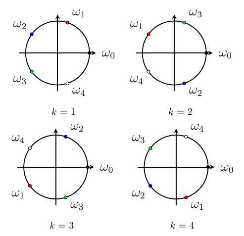
ELI5, the $N$-th roots of unity are the roots to the equation $\omega^N = 1$, which are $x_i = \omega^i$ where $\omega = \cos\left(\frac{2\pi}{N}\right) + i \sin\left(\frac{2\pi}{N}\right)$. In visual terms, by representing the complex numbers on a Cartesian plane, these roots of unity will be evenly spaced within a unit circle (and therefore forming a regular polygon with $N$ sides).

Earlier, it was mentioned that we only need to find half as many value as we needed previously. If the selected values to represent $P$ are $x_0, x_1, \ldots, x_{N-1}$, then we only need to find $x_0, x_1, \ldots, x_{\frac{N}{2}-1}$ and then we set the other half to be the negation of the first half. For example,

$$x_\frac{N}{2} = -x_0, x_{\frac{N}{2}+1} = -x_1, \ldots, x_{N-1} = -x_{\frac{N}{2}-1}$$

In order for the recursion to work, going from $x_0, x_1, \ldots, x_{N-1}$ representing $P$ to $x_0^2, x_1^2, \ldots, x_{\frac{N}{2}-1}^2$ representing $Q$ and $R$, the property should still hold: we can somehow find a way to pair

$$\left\{x_0^2, x_1^2, \ldots, x_{\frac{N}{2}-1}^2\right\} = \left\{\pm x_0^2, \pm x_1^2, \ldots, \pm x_{\frac{N}{4}-1}^2\right\}$$

based on their magnitudes but opposing signs. The term $x_i^2$ possibly being negative motivates us to use complex numbers for the $x_i$'s.

Take a small example of $P(x) = x^4 + x^3 + x^2 + x + 1$, a polynomial of degree 4. Since we need to find 5 points, we can extend this to finding $N = 2^{\lceil\log_2(5)\rceil} = 8$ points, namely

$$x_0, x_1, x_2, x_3, x_4=-x_0, x_5=-x_1, x_6=-x_2, x_7=-x_3$$

But we must have $x_2^2 = -x_0^2, x_3 = -x_1^2$, so we now need to find

$$x_0, x_1, x_2=\pm x_0 \cdot i, x_3=\pm x_1 \cdot i, x_4=-x_0, x_5=-x_1, x_6=\mp x_0 \cdot i, x_7=\mp x_1 \cdot i$$

But then, we must also have $x_1^4 = -x_0^4$. In the end, we must have

$$x_0^8 = x_1^8 = \ldots = x_7^8$$

Generalizing this idea for any value of $N$, we can select $x_0, x_1, \ldots, x_{N-1}$ such that

$$x_0^N = x_1^N = \ldots = x_{N-1}^N$$

In order to ensure these $N$ values are distinct, we make use of the $N$-th roots of unity by setting this common value to 1, resulting in $x_i = \omega^i, \forall 0 \le i < N$.

The FFT algorithm

Based on the previous points, we want to use recursion. But some questions remained unanswered: now that we derived $x_i = \omega^i$, how do we compute $p(x_i)$ for some polynomial $p$ efficiently for every recursion step?

Let's say we start with the polynomial $P(x)$ with coefficients $[a_0, a_1, a_2, \ldots, a_N]$. Divide into even and odd functions.

$$P(x) = E(x) + O(x) = Q(x^2) + xR(x^2)$$

This way, we can obtain $$Q(x) = [a_0, a_2, a_4, \ldots, a_{N-2}]$$ and $$R(x) = [a_1, a_3, a_5, \ldots, a_{N-1}].$$

Note that $N$ has been set to be a power of 2, so that the number of coefficients in $Q(x)$ is always the same as $R(x)$, and the way we divide the coefficients above tells us how to divide the input polynomial into two smaller ones, so someting like

$$\text{FFT}([a_0, a_1, a_2, \ldots, a_N]) = \text{merge}(\text{FFT}([a_0, a_2, a_4, \ldots, a_{N-2}]), \text{FFT}([a_1, a_3, a_5, \ldots, a_{N-1}]))$$

The next part is to determine how to merge the two FFT calls back into the final result.

Note that $\omega^{i+\frac{N}{2}} = -\omega^i$, so we will pair $x_i$ with $x_{i+\frac{N}{2}}$. Subsequently, we will pair $x_0$ with $x_\frac{N}{2} = -x_0$, $x_1$ with $x_{\frac{N}{2}+1} = -x_1$, and so on. But since we want to maintain the pairing when we recurse into the two halves, we have to take $x_0, x_2, x_4, \ldots, x_{N-1}$ as the values to compute (or alternatively only the odd indices, but this is less simpler).

To put it simply, if $\text{FFT}([a_0, a_1, a_2, \ldots, a_n])$ evaluates the polynomial at $$x = 1, \omega, \omega^2, \ldots, \omega^{N-1}$$ where $\omega^N = 1$, then $\text{FFT}([a_0, a_2, a_4, \ldots, a_{n-2}])$ and $\text{FFT}([a_1, a_3, a_5, \ldots, a_{n-1}])$ will evaluate the polynomial at $$x = 1, \omega^2, \omega^4, \ldots, \omega^{N-2}.$$

The plus-minus pairing is consistent since if $x_i$ is included in the subcase, so does $x_{i+\frac{N}{2}} = -x_i$ due to the parity of $\frac{N}{2}$ being even, with the exception of $N = 2$ (where it would be the base case and we only need to compute when $x = 1$).

Going back to our decompsition $P(x) = Q(x^2) + xR(x^2)$. Suppose we already have the evaluation results $$y_Q = [Q(1), Q(\omega^2), Q(\omega^4), \ldots, Q(\omega^{N-2})]$$ and $$y_R = [R(1), R(\omega^2), R(\omega^4), \ldots, R(\omega^{N-2})].$$

We can combine both $y_Q$ and $y_R$ to evaluate $P$ and end up with the array $y_P$ of length $N$.

$$ \begin{align*} y_P[i] = P(\omega^i) &= Q(\omega^{2i}) + \omega^i R(\omega^{2i}) \\ &= y_Q[i] + \omega^i y_R[i] \\ y_P\left[i+\frac{N}{2}\right] = P(\omega^{i+\frac{N}{2}}) = P(-\omega^i) &= Q(\omega^{2i}) - \omega^i R(\omega^{2i}) \\ &= y_Q[i] - \omega^i y_R[i] \\ \end{align*} $$

And thus we have obtained our final algorithm.

The runtime of this algorithm is defined by $T(n) = 2T(\frac{n}{2}) + O(n)$, which means $T(n) = O(n \log n)$. The $O(n)$ intermediate step is on the merging step and the construction of the two smaller arrays to recurse into.

If you want a numerical example of how this works, Reducible has once again cooked with this video.

Inverse FFT (IFFT)

Now that we have obtained the FFT algorithm that converts coefficient representation to value representation efficiently, if we want to multiply two polynomials $A(x)$ and $B(x)$ to obtain a polynomial $P(x)$ of degree $n$, we can just run $FFT(A) \rightarrow y_A$ and $FFT(B) \rightarrow y_B$, and then multiply the values element-wise to become $$y_P = [y_A[0] \cdot y_B[0], y_A[1] \cdot y_B[1], \ldots, y_A[n-1] \cdot y_B[n-1]].$$

But there is yet another question unanswered: how do we convert back $y_P$ to the coefficient representation of $P$?

Note that given $y_P$ and $\omega$ we can model this as a matrix equation.

$$ \begin{bmatrix} y_P[0] \\ y_P[1] \\ y_P[2] \\ \vdots \\ y_P[n-1] \\ \end{bmatrix} = \begin{bmatrix} 1 & 1 & 1 & \cdots & 1 \\ 1 & \omega & \omega^2 & \cdots & \omega^{n-1} \\ 1 & \omega^2 & \omega^{2 \cdot 2} & \cdots & \omega^{2(n-1)} \\ \vdots & \vdots & \vdots & \ddots & \vdots \\ 1 & \omega^{n-1} & \omega^{2(n-1)} & \cdots & \omega^{(n-1)(n-1)} \\ \end{bmatrix} \cdot \begin{bmatrix} a_0 \\ a_1 \\ a_2 \\ \vdots \\ a_{n-1} \\ \end{bmatrix} $$

The square matrix in that equation is called the Discrete Fourier Transform (DFT) matrix, and the inverse of that matrix is defined below. You are free to verify the correctness in your own time.

$$ {\begin{bmatrix} 1 & 1 & 1 & \cdots & 1 \\ 1 & \omega & \omega^2 & \cdots & \omega^{n-1} \\ 1 & \omega^2 & \omega^{2 \cdot 2} & \cdots & \omega^{2(n-1)} \\ \vdots & \vdots & \vdots & \ddots & \vdots \\ 1 & \omega^{n-1} & \omega^{2(n-1)} & \cdots & \omega^{(n-1)(n-1)} \\ \end{bmatrix}}^{-1} = \frac{1}{n}\begin{bmatrix} 1 & 1 & 1 & \cdots & 1 \\ 1 & \omega^{-1} & \omega^{-2} & \cdots & \omega^{-(n-1)} \\ 1 & \omega^{-2} & \omega^{-2 \cdot 2} & \cdots & \omega^{-2(n-1)} \\ \vdots & \vdots & \vdots & \ddots & \vdots \\ 1 & \omega^{-(n-1)} & \omega^{-2(n-1)} & \cdots & \omega^{-(n-1)(n-1)} \\ \end{bmatrix} $$

Therefore, we can obtain the solution to the equation which is

$$ \begin{bmatrix} a_0 \\ a_1 \\ a_2 \\ \vdots \\ a_{n-1} \\ \end{bmatrix} = \frac{1}{n}\begin{bmatrix} 1 & 1 & 1 & \cdots & 1 \\ 1 & \omega^{-1} & \omega^{-2} & \cdots & \omega^{-(n-1)} \\ 1 & \omega^{-2} & \omega^{-2 \cdot 2} & \cdots & \omega^{-2(n-1)} \\ \vdots & \vdots & \vdots & \ddots & \vdots \\ 1 & \omega^{-(n-1)} & \omega^{-2(n-1)} & \cdots & \omega^{-(n-1)(n-1)} \\ \end{bmatrix} \cdot \begin{bmatrix} y_P[0] \\ y_P[1] \\ y_P[2] \\ \vdots \\ y_P[n-1] \\ \end{bmatrix} $$

Take a close look at the above equation and compare it with the original equation system. Do you see a resemblance?

The original equation is transforming the coefficients of $P$ by FFT into $y_P$ using $\omega$. The above equation can therefore be seen as transforming $y_P$ by FFT into the coefficients of $p$ using $\omega^{-1}$, then we divide this result by $n$ due to the $\frac{1}{n}$ factor. Hence, the inverse FFT is just FFT with slightly different parameters!

Suppose the coefficient arrays that we want is $c_P$ and we have obtained $c_Q$ and $c_R$ through recursion, the merging step is very similar that of the normal FFT.

$$ \begin{align*} c_P[i] &= c_Q[i] + \omega^{-i} c_R[i] \\ c_P\left[i+\frac{N}{2}\right] &= c_Q[i] - \omega^{-i} c_R[i] \\ \end{align*} $$

In pseudocode form, the following.

The runtime of the algorithm is the same as the normal FFT. It is important to note that we still have to divide $c_P$ by $N$ to get the actual polynomial $P$.

Python code

Let's assume that we have implemented FFT and IFFT. We can code our multiplication function first.

def mult(p1, p2):
    m = len(p1)+len(p2)-1   # the actual degree of the product
    n = 2**(len(bin(m))-2)  # smallest power of 2 greater than m

    # pad both polynomials with zeroes to make them of length n
    p1_padded = p1 + [0]*(n-len(p1))
    p2_padded = p2 + [0]*(n-len(p2))

    # run FFT
    fft1 = fft(p1_padded)
    fft2 = fft(p2_padded)

    # combine and run IFFT
    values = [fft1[i]*fft2[i] for i in range(n)]
    tmp = ifft(values)
    return [tmp[i]/n for i in range(m)] # we only need to take the first m values

Next up, implementing both FFT and IFFT. For a given $n$, we can define the $n$-th root of unity $\omega$ as $\cos(\frac{2\pi}{n}) + i \sin(\frac{2\pi}{n})$.

from math import *

# put mult(p1, p2) here

def fft(p):
    n = len(p)
    if n == 1: return p # base case

    yq = fft(p[::2])    # even degrees
    yr = fft(p[1::2])   # odd degrees

    yp = [0]*n
    w = complex(cos(2*pi/n), sin(2*pi/n)) # n-th root of unity

    for i in range(n//2):
        yp[i] = yq[i] + w**i * yr[i]
        yp[i+n//2] = yq[i] - w**i * yr[i]
    return yp

def ifft(p):
    n = len(p)
    if n == 1: return p # base case

    cq = ifft(p[::2])   # even degrees
    cr = ifft(p[1::2])  # odd degrees

    cp = [0]*n
    w = complex(cos(2*pi/n), sin(2*pi/n)) # n-th root of unity

    for i in range(n//2):
        cp[i] = cq[i] + w**-i * cr[i]
        cp[i+n//2] = cq[i] - w**-i * cr[i]
    return cp

# demo
A = [1, 0, 5] # 5x^2 + 1
B = [1, 1]    # x + 1
print(mult(A, B)) # [(1+0j), (0.9999999999999998-2.2776579365114115e-16j), (5-1.6653345369377343e-16j), (5-1.6081226496766364e-16j)]

From the code above we can see a few rooms for improvement:

1. The computation of $\omega^i$ can be optimized by multiplying a variable by $\omega$ every iteration and use that variable instead.
2. FFT and IFFT can be generalized into a single function, so we only need to specify the multiplier: $\omega$ or $\omega^{-1}$.
3. The result is very prone to floating point errors, which why we might want to simply take the real component of the IFFT values in order to reduce the noise. Rounding of the real component might be useful if you are dealing with only integer coefficients.

Next, we can come up with something like the following.

from math import *

def mult(p1, p2):
    m = len(p1)+len(p2)-1   # the actual degree of the product
    n = 2**(len(bin(m))-2)  # smallest power of 2 greater than m

    # pad both polynomials with zeroes to make them of length n
    p1_padded = p1 + [0]*(n-len(p1))
    p2_padded = p2 + [0]*(n-len(p2))

    # run FFT
    fft1 = fft(p1_padded, False)
    fft2 = fft(p2_padded, False)

    # combine and run IFFT
    values = [fft1[i]*fft2[i] for i in range(n)]
    tmp = fft(values, True)
    return [round(tmp[i].real/n, 9) for i in range(m)] # we only need to take the first m values

def fft(p, inv):
    n = len(p)
    if n == 1: return p     # base case

    yq = fft(p[::2], inv)   # even degrees
    yr = fft(p[1::2], inv)  # odd degrees

    yp = [0]*n
    w = complex(cos(2*pi/n), sin(2*pi/n)) # n-th root of unity
    if inv: w = 1/w
    wi = 1

    for i in range(n//2):
        yp[i] = yq[i] + wi * yr[i]
        yp[i+n//2] = yq[i] - wi * yr[i]
        wi *= w
    return yp

# demo
A = [1, 0, 5] # 5x^2 + 1
B = [1, 1]    # x + 1
print(mult(A, B)) # [1.0, 1.0, 5.0, 5.0]

You can convert the FFT recursion into an iterative one. In the example below, I'm using cmath rather than math, so I can optimize a few things to a minor extent. As a result, defining $\omega$ will require Euler's formula $\omega = e^{\frac{\pm 2 \pi i}{n}}$. If you need to refresh on how to convert a recursion to iterative, you can check out this article I made earlier.

from cmath import *
def fft(v, inv=False):
    stack = [(2*len(v), v)]; tmp = []
    while stack:
        nb, v = stack.pop(); n, b = nb//2, nb%2
        if b == 0:
            if n == 1: tmp.append(v)
            else: stack.append((2*n+1, v)), stack.append((n, v[1::2])), stack.append((n, v[::2]))
        else:
            yo, ye = tmp.pop(), tmp.pop(); y, wj = [0]*n, 1; w = exp(-1j*(2-4*inv)*pi/n)
            for i in range(n//2): y[i] = ye[i]+wj*yo[i]; y[i+n//2] = ye[i]-wj*yo[i]; wj *= w
            tmp.append(y)
    return tmp[0]

You can also make the array operations in-place. The explanation is out-of-scope of the article, so you can check the full code for more details.

FFT and 3-SUM

There are so many Kattis questions that make use of FFT, but the simplest application of FFT other than polynomial multiplication would be the well-known 3-SUM problem.

Given $n$ integers $x_1, x_2, \ldots, x_n$ where $x_i \in [-N, N]$ and a target number $T$. We want to check if there are 3 numbers summing up to $T$. While the usual solution makes use of a hashmap and runs in $O(n^2)$ time, we can use FFT to solve this in $O(n + N \log N)$ time, which might be faster for sufficiently small values of $N$.

Represent the $n$ integers as a polynomial $P(x) = a_0 + a_1 x + a_2 x^2 + \ldots + a_{2N} x^{2N}$ where $a_i$ is the frequency of $i-N$ in the set. Then, we compute $P(x)^2$ using FFT to represent all possible pair sums of the $n$ integers.

Suppose the product is $Q(x) = b_0 + b_1 x + b_2 x^2 + \ldots + b_{4N} x^{4N}$. Notice that if we have two numbers $i$ and $j$, their sum, $i+j$, will contribute to the coefficient of $x^{i+N} \cdot x^{j+N} = x^{i+j+2N}$. This means we just need to find for each of the $n$ integers $x_i$, whether $T - x_i$ is present, which suffices to check if the coefficient of $T - x_i + 2N$ is nonzero.

Do take note of the case when they're asking for distinct integers, in which we have to subtract $Q(x)$ on the terms where the $2x_i$'s can contribute. A similar problem with this consideration also exists on Kattis: A+B Problem.

Now that it can solve 3-SUM, we can generalize FFT to be able to deal with convolutions: it's not just polynomial multiplication or 3-SUM, but rather problems with sum over aligned pairs, something in the form of

$$C[k] = \sum_i A[i] \cdot B[k-i]$$

Number Theoretic Transform (NTT)

ELI5, it's FFT but without involving any complex numbers, but rather prime numbers. The idea is that instead of using the $n$-th root of unity, $\omega$, we choose a sufficiently large prime number $M$ and then work on modulo $M$.

Primitive roots

To get started, we need to understand about primtive roots modulo $n$.

According to Wikipedia, a number $g$ is a primitive root modulo $n$ if for every number $a$ coprime to $n$, we can find an integer $k$ such that $g^k \equiv a \pmod n$. Using Euler's theorem we can rephrase such that $g$ is a primitive root modulo $n$ if and only if $g^{\phi(n)} \equiv 1 \pmod n$ but $g^k \not\equiv 1 \pmod n$ if $k < \phi(n)$, where $\phi(n)$ is the Euler's totient function that computes the number of positive up to $n$ that are coprime to $n$.

A primitive root exists if and only if $n$ is in the form of $1, 2, 4, p^k,$ or $2p^k$ where $p$ is an odd prime and $k \ge 1$. The proof is out of scope, since only need to deal with $n$ being a large prime number.

As a side, one can find the primitive root modulo $n$ using this Python code.

# Eratosthenes prime sieve
LIMIT = 10**6
spf = list(range(LIMIT+1))
primes = [2]; p = 3
while p <= LIMIT:
    if spf[p] == p:
        primes.append(p)
        for i in range(p*p, LIMIT+1, 2*p):
            if spf[i] == i: spf[i] = p
    p += 2

# Prime factorization
# Alternatively you can also backtrack using Pollard-Rho
def prime_factorization(n):
    res = {}; idx = k = 0
    while n != 1 and idx < len(primes):
        pp = primes[idx]
        if pp*pp > n: break
        if n % pp == 0:
            while n % pp == 0: n //= pp; k += 1
            res[pp] = k
        idx += 1; k = 0
    if n != 1: res[n] = 1
    return res

from math import gcd
def find_primitive_root(n):
    p = prime_factorization(n)
    if n in (1, 2, 4) or len(p) == 1 or (p.get(2, 0) == 1 and len(p) == 2): # check if it's in the form of 1, 2, 4, p^k, 2p^k
        # compute t = phi(n)
        t = n
        for i in p: t = t//i*(i-1)
        # just need to work on prime factors of t
        q = prime_factorization(t)
        for i in range(n):
            if gcd(i, n) == 1 and 1 not in {pow(i, t//j, n) for j in q} and pow(i, t, n) == 1: return i
    return None

# Test
print(find_primitive_root(998244353))

The algorithm

First, we need a prime number $p = k \cdot n + 1$, where $k$ is a positive integer and $n$ is the number of coefficients in the input polynomial.

This is why $998244353 = 119 \cdot 2^{23} + 1$ is one of the most frequently used prime number besides $10^9 + 7$: we can easily bring $n$ to a power of 2 so that for such values of $n$, the value $k = \frac{119 \cdot 2^{23}}{n}$ is definitely a valid integer. Moreover, $3$ is a primitive root of $998244353$.

Suppose $g$ is a primitive root modulo $p$. Therefore, $g^{p-1} \equiv 1 \pmod p$ but $g^k \not\equiv 1 \pmod p$ if $k < p-1$. All of these $g^k$'s must have a different modulo for $k = 1, 2, \ldots, p-2$. Otherwise, we can find two values $i \le j$ such that $g^i \equiv g^j \pmod p$ and therefore $g^{j-i} \equiv 1 \pmod p$ but $j-i < p-1$, a contradiction.

Now, define $\omega = g^k \pmod p$. We have $$\omega^n = g^{kn} = g^{p-1} \equiv 1 \pmod p,$$ but $$\omega^i = g^{ik} \not\equiv 1 \pmod p, \forall 1 \le i < n$$ because $ik < p-1$ and all of the $\omega^i$'s are different modulo $p$ based on our previous argument. Therefore $\omega$ is a valid $n$-th root of unity modulo $p$.

We can then run the usual recursion but work in modulo $p$. The pairing is exactly the same since $\omega^{\frac{n}{2}} \equiv -1 \pmod p$.

Python code

Let's review the original FFT recursion.

from math import *

def mult(p1, p2):
    m = len(p1)+len(p2)-1
    n = 2**(len(bin(m))-2)

    p1_padded = p1 + [0]*(n-len(p1))
    p2_padded = p2 + [0]*(n-len(p2))

    fft1 = fft(p1_padded, False)
    fft2 = fft(p2_padded, False)

    values = [fft1[i]*fft2[i] for i in range(n)]
    tmp = fft(values, True)
    return [round(tmp[i].real/n, 9) for i in range(m)]

def fft(p, inv):
    n = len(p)
    if n == 1: return p

    yq = fft(p[::2], inv)
    yr = fft(p[1::2], inv)

    yp = [0]*n
    w = complex(cos(2*pi/n), sin(2*pi/n))
    if inv: w = 1/w
    wi = 1

    for i in range(n//2):
        yp[i] = yq[i] + wi * yr[i]
        yp[i+n//2] = yq[i] - wi * yr[i]
        wi *= w
    return yp

# demo
A = [1, 0, 5] # 5x^2 + 1
B = [1, 1]    # x + 1
print(mult(A, B)) # [1.0, 1.0, 5.0, 5.0]

We can modify FFT to NTT by setting the big prime number as the modulo, say $M = 998244353$, and then use the primitive root $g = 3$ to determine the value of $\omega = g^k = g^{\frac{M-1}{n}}$.

M = 998244353
g = 3 # or you can run find_primitive_root(M) defined above

def mult(p1, p2):
    m = len(p1)+len(p2)-1
    n = 2**(len(bin(m))-2)

    p1_padded = p1 + [0]*(n-len(p1))
    p2_padded = p2 + [0]*(n-len(p2))

    ntt1 = ntt(p1_padded, False)
    ntt2 = ntt(p2_padded, False)

    values = [ntt1[i]*ntt2[i]%M for i in range(n)]
    tmp = ntt(values, True)
    inv_n = pow(n, -1, M)
    return [ntt[i]*inv_n%M for i in range(m)]

def ntt(p, inv):
    n = len(p)
    if n == 1: return p

    yq = ntt(p[::2], inv)
    yr = ntt(p[1::2], inv)

    yp = [0]*n
    w = pow(g, (M-1)//n, M)
    if inv: w = pow(w, -1, M)
    wi = 1

    for i in range(n//2):
        yp[i] = yq[i] + wi * yr[i]
        yp[i+n//2] = yq[i] - wi * yr[i]
        wi = wi*w%M
    return yp

# demo
A = [1, 0, 5] # 5x^2 + 1
B = [1, 1]    # x + 1
print(mult(A, B)) # [1, 1, 5, 5]

The runtime is the same as FFT or IFFT, which is $O(n \log n)$ where $n$ is the degree of the polynomial. However, it should have a less constant factor due to the simpler arithmetic operations as compared to complex numbers. NTT is also more robust against floating point errors because such errors won't happen here - we're using integers and only integers.

If you need even higher primes you can try $9223372036737335297 = 2^{24} \cdot 549755813881 + 1$ or $2524775926340780033 = 2^{24} \cdot 150488372227 + 1$. They are both prime numbers with $3$ as a primitive root of that modulo.

You can also convert the recursive NTT to iterative the same way that I did on FFT. There are many variations to these, and the heavily optimized ones can be found at the Yosupo judge, specifically the two submissions: here and here. The Python version of the two Yosupo codes can be found at pytils since I have been using it for some Kattis problems: Number Theoretic Transform and Dice Results.

Bonus: Polynomial Division

The last section is heavily inspired by the Kattis problem Dice Distributions: given three polynomials $A, B, C$, find the polynomial $D$ such that $A \cdot B = C \cdot D$. Multiplying $A$ and $B$ is now a rather simple task using FFT or NTT, but how do we divide it by $C$?

The research paper from Cao and Cao and this lecture notes from Thibaut Verron were great inspirations on implementing polynomial division.

Inversion by Newton iteration

Given a polynomial $P(x)$ of degree $n$, we want to find another polynomial $Q(x)$ such that $P(x)Q(x) \equiv 1 \pmod {x^l}$ for a sufficiently large value of $l$, and how this was basically done is using Newton iteration. We can set $l$ to be the next power of 2 larger than $n$, similar to FFT.

In short, the algorithm is as follows.

For example, I want to invert $P(x) = -5x^4 + 3x^3 - 7x^2 + 6x + 3 = [3, 6, -7, 3, -5]$.

1. Start with $v = [\frac{1}{3}]$.
2. $N = 8$, so I will repeat Step 2 of the algorithm for 3 times.
   • $i = 1, v = 2v-Pv^2 \pmod {x^2}$ $$\begin{align*} v &= 2 \cdot \left[\frac{1}{3}\right] - \left[3, 6\right] \cdot \left[\frac{1}{3}\right]^2 \pmod {x^2} \\ &= \left[\frac{2}{3}-\frac{3}{9}, -\frac{6}{9}\right] \pmod {x^2} \\ &= \left[\frac{1}{3}, -\frac{2}{3}\right] \end{align*}$$
   • $i = 2, v = 2v-Pv^2 \pmod {x^4}$ $$\begin{align*} v &= 2 \cdot \left[\frac{1}{3}, -\frac{2}{3}\right] - \left[3, 6, -7, 3\right] \cdot \left[\frac{1}{3}, -\frac{2}{3}\right]^2 \pmod {x^4} \\ &= \left[\frac{2}{3}, -\frac{4}{3}\right] - \left[3, 6, -7, 3\right] \cdot \left[\frac{1}{9}, -\frac{4}{9}, \frac{4}{9}\right] \pmod {x^4} \\ &= \left[\frac{2}{3}, -\frac{4}{3}\right] - \left[\frac{1}{3}, -\frac{2}{3}, -\frac{19}{9}, \frac{55}{9}, -\frac{40}{9}, \frac{4}{3}\right] \pmod {x^4} \\ &= \left[\frac{1}{3}, -\frac{2}{3}, \frac{19}{9}, -\frac{55}{9}\right] \end{align*}$$
   • $i = 3, v = 2v-Pv^2 \pmod {x^8}$ $$\begin{align*} v &= 2 \cdot \left[\frac{1}{3}, -\frac{2}{3}, \frac{19}{9}, -\frac{55}{9}\right] - \left[3, 6, -7, 3, -5\right] \cdot \left[\frac{1}{3}, -\frac{2}{3}, \frac{19}{9}, -\frac{55}{9}\right]^2 \pmod {x^8} \\ &= \left[\frac{2}{3}, -\frac{4}{3}, \frac{38}{9}, -\frac{110}{9}\right] - \left[3, 6, -7, 3, -5\right] \cdot \left[\frac{1}{9}, -\frac{4}{9}, \frac{50}{27}, -\frac{62}{9}, \frac{1021}{81}, -\frac{2090}{81}, \frac{3025}{81}\right] \pmod {x^8} \\ &= \left[\frac{2}{3}, -\frac{4}{3}, \frac{38}{9}, -\frac{110}{9}\right] - \left[\frac{1}{3}, -\frac{2}{3}, \frac{19}{9}, -\frac{55}{9}, -\frac{496}{27}, \frac{488}{9}, -\frac{13036}{81}, \frac{38633}{81}\right] \pmod {x^8} \\ &= \left[\frac{1}{3}, -\frac{2}{3}, \frac{19}{9}, -\frac{55}{9}, \frac{496}{27}, -\frac{488}{9}, \frac{13036}{81}, -\frac{38633}{81}\right] \end{align*}$$
3. So the inverse is the polynomial $$Q(x) = -\frac{38633}{81}x^7 + \frac{13036}{81}x^6 -\frac{488}{9}x^5 + \frac{496}{27}x^4 -\frac{55}{9}x^3 + \frac{19}{9}x^2 -\frac{2}{3}x + \frac{1}{3},$$ indeed a lot of fractions, but $$P(x)Q(x) = \frac{193165}{81}x^{11} - \frac{181079}{81}x^{10} + \frac{331499}{81}x^{9} - \frac{343666}{81}x^{8} + 1 \equiv 1 \pmod {x^8}$$ as expected.

The division algorithm

Once we understand the inversion, the division algorithm is rather straightforward. Suppose we want to divide the polynomial $P(x)$ by $Q(x)$.

Originally, one would've done the following.

• If $\deg(P) < \deg(Q)$, the quotient is $0$ and the remainder is $P$ itself.
• Let $m = \deg(P) - \deg(Q)$ and $n$ be the smallest power of 2 greater than $m$.
• Compute $Q^{-1} \pmod {x^n}$ using Newton iteration.
• The quotient, $q$, is $PQ^{-1} \pmod {x^{m+1}}$.
• The remainder, $r$, is therefore equal to $P-qQ$.

However, this approach is not always effective. The reason is that when you want to invert $Q$, you have to make sure that the constant $Q_0$ is non-zero. Since the leading coefficient is definitely non-zero, we can work on the reversed coefficients of the polynomial. In short, we define the $n$-th reversal of a polynomial $P$ of degree $n$ as

$$\text{rev}_n(P) = x^n P\left(\frac{1}{x}\right)$$

For example, if $P(x) = 2x^3 + 3x^2 - 7x$, then $\text{rev}_3(P) = x^3 (\frac{2}{x^3} + \frac{3}{x^2} - \frac{7}{x}) = 2 + 3x - 7x^2$. In Python array terms, we have

$$\text{rev}_3([0, -7, 3, 2]) = [2, 3, -7, 0]$$

Now, we can slightly modify our division algorithm to be like this (the modulo is slightly modified from the one defined by Thibaut Verron for convenience).

Assuming the multiplication takes $O(n \log n)$ time for polynomials of degree $n$. The time complexity of the division algorithm is as follows:

• Suppose the degree of $P$ is $n$. If $\deg(Q) > n$, we are done, so the full algorithm happens when $\deg(Q) \le n$. Therefore,reversing $P$ and $Q$ to be $R$ and $S$ takes $O(n)$ time.
• Computing the inverse of $S$ takes $\log n$ iterations of the update $$2v - Sv^2 \pmod {x^{2^i}},$$ where on iteration $i$, the multiplication takes $O(2^i \log {2^i})$ time. Therefore, the total runtime on this step is $$ \begin{align*} O\left(\sum_{i=1}^{\log n} 2^i \log 2^i \right) &= O\left(\sum_{i=1}^{\log n} i \cdot 2^i \right) \\ &= O\left(\sum_{i=1}^{\log n} 2^i + \sum_{i=2}^{\log n} 2^i + \ldots + \sum_{i=\log n}^{\log n} 2^i \right) \\ &= O\left(\sum_{i=0}^{\log n - 1} 2^i + \sum_{i=1}^{\log n - 1} 2^i + \ldots + \sum_{i=\log n - 1}^{\log n - 1} 2^i \right) \\ &= O\left((2^{\log n} - 2^0) + (2^{\log n} - 2^1) + \ldots + (2^{\log n} - 2^{\log n - 1}) \right) \\ &= O\left(\log n 2^{\log n} - (2^0 + 2^1 + \ldots + 2^{\log n - 1}) \right) \\ &= O\left(n \log n - 2^{\log n} + 1 \right) \\ &= O\left(n \log n \right). \end{align*} $$
• Computing $RS^{-1}$ and reversing it takes $O(n \log n)$ time.
• Computing the remainder also takes $O(n \log n)$ time due to the multiplication $qQ$.

Overall, the algorithm takes $O(n \log n)$ time, where $n$ is the degree of $P$.

Python code

# Assume the function mult(u, v) has been defined earlier
# Whether FFT or NTT, adjust the arithmetic operations accordingly
# In this code, assume FFT is the one used

# Subtract two polynomials u-v
def sub(u, v):
    z = [*u]
    while len(z) < len(v):
        z.append(0)
    for i in range(len(v)):
        z[i] -= v[i]
    while z[-1] == 0:
        z.pop()
    return z

def div(P, Q):
    # Cleanup zero leading coefficients
    while P and P[-1] == 0: P.pop()
    while Q and Q[-1] == 0: Q.pop()

    # Reverse both P and Q to u and v
    u = P[::-1]
    v = Q[::-1]

    # Newton's iteration
    vi = [1/v[0]]
    n = len(u)-len(v)+1
    p = 1
    w = [] # to store v mod x^p
    while p < n:
        p *= 2

        # populate [v mod x^(p_new)] - [v mod x^(p_old)] to w
        while len(w) < min(p, len(v)):
            w.append(v[len(w)])

        # q_i = v_i * v_i * w, and then (optionally?) remove zero leading coefficients of w
        qi = mult(mult(vi, vi), w)
        while len(w) > min(p, len(v)) and w[-1] == 0:
            w.pop()

        # compute v_i = 2*v_i - q_i
        while len(vi) < p:
            vi.append(0)
        for i in range(len(vi)):
            vi[i] *= 2
        vi = sub(vi, qi)

    # Wrap-up
    z = mult(u, vi)[:n]
    return z[::-1] # reverse again

# Demo time!
# Expected: 14x/3 + 13/9 with remainder of -34x/9 + 109/9, plus some floating point errors
A = [15, 7, 9, 14]  # 14x^3 + 9x^2 + 7x + 15
B = [2, 1, 3]       # 3x^2 + x + 2
Z = div(A, B)
print('Quotient:', Z)
print('Remainder:', sub(A, mult(B, Z)))

# Second demo
# Expected: x^2 - 1 with remainder of x^3 - 1
A = [-1, 0, 0, 0, 0, 0, 0, 1]   # x^7 -1
B = [0, 0, 0, 1, 0, 1, 0, 0]    # x^3 + x^5 but with some zero leading coefficients
Z = div(A, B)
print('Quotient:', Z)
print('Remainder:', sub(A, mult(B, Z)))

Challenge: If I don't use reversion (i.e. let $u = P, v = Q$ and then just return $z$), the algorithm seems to work only when the remainder is zero, but not so much otherwise. Can you find out why?

For reference, check out the heavily-modified version of the code that works for divisions that leave no remainder.